GIS I Mini Term Project

Mini-Term Project

                The main goal of this project is to help me understand how GIS can be employed to solve practical problems in a study area of my choice. The project entails identifying and developing a problem that has spatial dimension, generate certain criteria that can be used in solving the problem, and outline data types and methods that I will engage in executing the project. The project will consist of a simple spatial question, which in this report I choose to discuss where the best place to put a new cabin.

                This spatial question is designed to reach out to people interested in investing in a cabin and finding the best site for a cabin can be a tough, hard decision, but I have created a criteria that I believe will be the best fit for the perfect location. The study area I selected is the northern counties of Wisconsin because most people are looking for a location up north where some of the most beautiful forests, lakes, and rivers that offer endless opportunities to enjoy the area. The activities include fishing, boating, canoeing, hiking, hunting, snowshoeing, cross-country skiing, sightseeing snowmobiling, and ATV trail riding. This project is important to people who are strongly thinking about investing in a cabin because owning a cabin is a valuable, significant commitment.

                Within the northern counties of Wisconsin I included lakes, forest, cities, and major roads. I determined that the lakes shapefile is my most important layer because most people prefer to have a cabin on a lake considering all the multiple activities you can enjoy. The forest shapefile includes both national forest and county forest. I found this layer the most interesting because almost all of the forest locations were located in the northern counties and takes up almost a quarter of the counties area, which suggest hiking and wild life are greatly appreciated as well as entertaining. I selected the cities shapefile because I wanted the location of the cabin to be near a city where goods and services can be accessed without having the fear of being in the middle of nowhere. The last shapefile, major roads, is included so people can easily reach their cabin locations without having the hassle of taking multiple back roads. I retrieved my data from our university’s database connection by connecting to Wisconsin’s Department of Natural Resources database and ESRI’s United States of America database. From Wisconsin’s DNR database I used Wisconsin’s county boundaries, major roads, national forest, county forest, and three lakes shapefiles. From ESRI’s USA database I only used the cities shapefile. The only data concern I had with the data I acquired was that the Wisconsin’s DNR database was missing some lakes, otherwise I was satisfied with my data.

                Many methods were used to answer my geospatial question. I first began with the Wisconsin county boundaries shapefile where I then created an sql expression to eliminate all counties except for the northern counties. Once I established my foundation of my map I brought in three separate lake shapefiles. Since the lake shapefiles were separate from each other I used my geoprocessing technique called union to ultimately combine the three shapefiles together. After preforming the union technique I created a sql that selected only lakes or flowages in the attribute table because I did not want to include ponds, springs, and swamps. Next I made an intersection of my new lakes shapefile with the northern counties so I could eliminate the lakes outside of the northern counties. The same techniques was applied to the national forest and the county forest shapefile. I performed the union geoprocessing procedure and then used the intersection process, which included the northern counties. Next I constructed a buffer around the new forest shapefile. I set the buffer distance to one mile and used the dissolve technique to lose the multiple lines that disrupted the visual effect on my map. The cities shapefile would ultimately determine the location of the cabin. When I first imported the city shapefile I had over 50 city points located inside the county shapefile and need to create a sql that would eliminate more than half and still make sense. The sql I created included the cities 2007 population that was greater than or equal to 2,500 people. I then intersected the new city layer with the northern county layer and established a 25 mile buffer around the city with also using the dissolve technique to lose lines that overlapped each other. I chose a 25 mile buffer around the 15 selected cities because I figured it would be best for getting quick access to the goods and services you need. To complete my map I finished with intersecting the forest buffer and city buffer so I could have more of a visual concentration on what matter, which is identifying the lakes present within the city as well as forest buffer.

As a result from my project I ended with a total of 19 lakes that met my criteria. To reiterate my criteria the location of my cabin has to be on a lake or flowage that is a mile away from a county or national forest with also being within a 25-mile buffer of a city greater than or equal to 2,500 people. The lakes that met the criteria are outlined in dark blue as well as label. Overall I am satisfied with my final map and I believe the benchmarks set are ideal along with a simple reflection of a great, enjoyable location. If I were to repeat this project I would try to look for more lake shapefiles to include and also tables that provided a field that reflected the lakes total area.

GIS I Lab 5

The main goal of lab five is to enable myself to appropriately choose and apply various vector geoprocessing tools encountered in lectures and Price tutorials to determine suitable habitats for bears in the study area of Marquette County, Michigan. In addition to my lab I was introduced to the ArcGIS python window and explored its functionalities in running geoprocessing operations by writing scripts.

            In part one of the lab I examined an attribute table that is based on GPS locations of black bears in Michigan and with that data I need to determine the forest types where blacks bears are found in central Marquette County. To determine the results I applied the intersecting geoprocessing tool, which ultimately combined the black bear location data and land cover data. As a result from the exercise I was able to determine that the number one forest type with black bears present is mix forest land. Next I determined black bears occurrence within a ten-mile proximity of streams in Marquette County. First I used the geoprocessing tool called buffer, which allows us to identify areas or features that fall within a certain distance of applied feature(s). After applying the buffer tool I dissolved the streams buffer, which combines the entire streams buffer into one by eliminating lines within the buffer making it more neat and organized. Once the buffer and dissolve process is complete, the black bear location shapefile is intersected with the stream buffer, dissolve shapefile. I found from the results of this data that 73% of the bears are located with a ten-mile buffer from a stream. My last task of part one was to include the DNR management areas in the study area of Marquette County. When first adding the DNR management areas I noticed that I needed to use the dissolve tool to eliminate lines within the boundaries of their designated areas. My next step was to then intersect the DNR management areas and study area, so I could remove DNR areas that didn’t apply to the study area. After implementing basic geoprocessing operations and creating a cartographically pleasing map in part one it was then time to move on to part two.

            Part two involved python scripting, which is first introduced to me to help prepare myself for advanced GIS courses. Objective one involved finding suitable areas for the development of tourist resorts in Wisconsin. The shapefiles used in part two are Wisconsin cities, interstates, lakes, and counties. To perform the first objective I opened the python window and began scripting for the first time. The first scripted line is import arcpy. My next line requires a buffer analysis on Wisconsin cities and dissolving the ten-mile buffer. My next task is to perform is the geoprocessing operation called clipping, so in my python window I do a clip analysis on lakes that are greater than five square miles within the ten-mile buffer of the cities. After completing the python scripting I have my results and can now determine where to develop a tourist resort. The second objective is to model air pollution impact zones along interstates in Wisconsin. Performing this analysis requires the use of the python window where I apply a multiple ring buffer to the interstates on mile one, two, three, four, five, and six. The closest buffer to the interstate is the most hazardous meaning very high air pollution and at the six-mile buffer there is a low amount of air pollution. Once both objectives in part two were complete I designed two pleasing, organized maps that can be analyzed easily by a viewers.

            The completion of lab five helped me appropriately apply numerous vector geoprocessing operations in python scripting to real life scenarios and benefited me by making fast as well as easy analysis on the projected data.

GIS 1 Lab 4

Lab 4

                  The main goal of this lab is to excise and develop my skills in composing as well as implementing query expressions to extract components of data from a database. This lab is intended to assess my understanding of attribute and spatial queries.

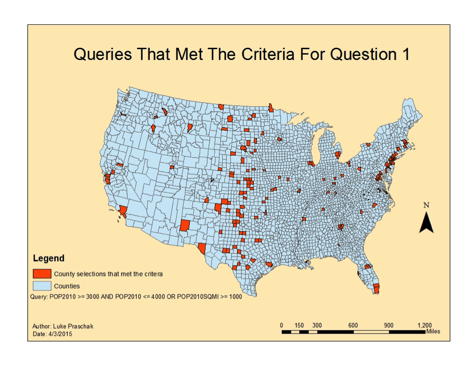
                  My first task in lab four, part one was to construct a multiple criteria query for the United States county shapefile. The query involved retrieving counties with a population between 3,000 and 4,000 people in 2010 and also including all counties in 2010 that had a population density of at least 1,000 persons per square mile. There was a total of a 194 counties, which included 32 states that met the criteria. Next I wrote a multiple criteria query that returned records for counties located in Wisconsin, Texas, Minnesota, New York, and California. The query I developed would include a greater male population than female and the number of seniors age 65 and above over 6,500. 46 counties within the five states were returned from the results and Texas had the highest number of counties at 15. The next exercise involved modifying the query above by adding all the other seniors age 65 and above in Washington, Maryland, Illinois, Nebraska, District of Columbia, and Michigan who resided in counties that have more than 30,000 housing units. 128 counties fulfilled the new query.

                  Part two of lab four was the most challenging and interesting project, which included a Wisconsin database. My first task is to develop a query that will return cities in Wisconsin with a 2007 population between 15,000 and 20,000 people, an area of the city that is at least five square miles in land area, the female population is greater than males, and also the cities are within two miles of a lake. Before performing the multiple criteria query I joined the lakes attribute table to the Wisconsin cities attribute table because that is the information I would need to help me determine which cities on the shapefile are located within two miles of a lake. After using the joining process I was now able to successfully project my data and get accurate results. There was total of eight cities that met this query’s criteria. My final task for part two is to create another multiple criteria query that will calculate the total length of 13 Wisconsin rivers. The distance of the rivers came to be around 700 miles.

                  Being able to create multiple criteria queries is an extremely important skill for retrieving GIS attribute data. Even though it takes time to learn the SQL language it is unique and fascinating to see how data can be returned to the user so quickly. This process makes analyzing, manipulating, and organizing data extremely easy as well as fast.

United States Question 1

United States Question 3

Wisconsin Cities

Wisconsin Rivers

GIS 1 Lab 3

The main objective for lab three is to continue practicing GIS and standalone data that can be used for analysis in a GIS project. The lab focused on converting standalone tables containing data into an attribute table that can be mapped and then exercised manipulating the U.S. Census Bureau’s website to acquire information to be used in a GIS.

            The U.S. Census Bureau website is first introduced and the mission of the bureau is to serve as the leading source of quality data about the nation’s people and economy. The data collected is used to regulate the distribution of Congressional seats to states, make decisions about what community services to provide as well as distributing $400 billion dollars in federal funds. Downloading the 2010 U.S. Census of Wisconsin by county is our first task followed by downloading the Wisconsin shapefile, which is also obtained from the website. Once the downloading and saving was complete modifications to the Excel spreadsheet involving Wisconsin’s counties population were made. Deleting an unneeded record, adjusting the population field’s decimal places, formatting the population field to numbers instead of text and finally saving the spreadsheet as an Excel workbook, which ultimately made it possible to add to ArcMap. Tying the Wisconsin shapefile and the spreadsheet together is the next task. The process used to combine the two is called the join technique. This technique helps link the census data and the shapefile into one attribute table. After applying the join method the data is now ready to be projected. Under symbology’s quantities graduated colors the selected value is population, which displays the most common used color ramp for population ranging from red (highest in density) to light yellow (lowest).  The classification method used is defined interval with five classes. I chose this classification method because I thought it best represented the distribution of population by county in Wisconsin.

            The next objective is to project data of our choice onto the Wisconsin county shapefile. Housing units was my selected variable. Following the same steps from the map created before I only changed the joining process. The joining process involved tying Wisconsin’s housing units and the population data table into the county’s shapefile. Once the joining technique was finished projecting the data was next on the list of steps. The map displays the population, which is divided by the number of housing units. I found this projection unique because the number of housing units in the northern counties exceeds the population. The data is projected this way because of the number of cabins present in the north. The classification method used is geometric interval. Once the maps were complete the essential elements of map design were added to ensure the viewer has a well understanding of the goal expressed.

            Downloading and mapping GIS data is an extremely important skill. I can now use data from a source outside of ArcMap. I’ve learned to convert along with join data tables as well as import shapefiles to project my data selected.

Source

 

American FactFinder. (2015, January 6). Retrieved March 12, 2015, from http://factfinder2.census.gov/faces/nav/jsf/pages/index.xhtml

 

 

GIS 1 Lab 1

The knowledge of fixing various coordinate systems is critical for designing maps because every map is deceiving in its own unique way. In our first lab we are asked to look more in depth, in recognizing the problems along with the benefits of each individual coordinate system have.

                First we are asked to add the world shape file to ArcMap and produce a particular projection of the world. This step is repeated four times with each map requiring a different world projection. The projections that I applied were the Mercator, Sinusoidal, Geographic, Equidistant-Conic, and Van der Grinten I. For this exercise the goal is to show the areas that are distorted and preserved across the map projection. Starting with the Mercator projection; here this projection helps preserve direction and shape, but distorts distance along with area. Notice once you move north or south from the equator the area steadily increases. The Mercator is a projection that is commonly used for world map. Next is the Sinusoidal, which helps preserve direction and shape, however distorts area and distance. This projection I find the most appealing because the viewer gets the correct impression of the relative geographic sizes of the continents, oceans, and countries. The geographic projection helps preserve the area and direction, but transforms the shape and distance. This map projection is excellent for pilot navigation. The most interesting applied projection is the Equidistant-Conic. I find this fascinating due to of the unique North Pole perspective you observe. Here we see maintained distance and area, but alters the direction and shape. My final projection I choose is the Van der Grinten I. I picked this projection because I thought the name was amusing and I also found out that the map projection shares the same characteristics as the Mercator projection. I find this better than the Mercator because I like how the cartographer constructed circular arcs for both meridians making its data on a global scale.

                After applying the five world projections I proceeded to make my own map projection of the United States of America and the state of Wisconsin. Here I used the U.S. was the GCS (geographic coordinate system) North America 1983 projection. Once the U.S. shapefile was established I then proceeded to add and fix the Michigan roads shapefile. As a result the projection reflected the overlay of the two shape files calling this an “On the fly projection.” The objective for Wisconsin is to change its projection to UTM, NAD 1983, Zone 16N. Where this helps keep distortion to a minimal. After completion of the two map projections we were obligated to join the five previous projections with the two recently applied projections onto one document. The finished product is shown in figure 1.

                The last exercise performed involved “On the fly projection.” This time the projection included the central Wisconsin counties and the present river ways. This exercise also implicated us to fix the coordinate system so the two different shape files could be compatible with each other. When come to completing the lesson I am asked again to fit the projection onto one document (figure 2) while having to add a legend, neat line, north arrow, and a scale.

                Finally the lab is complete. I can now evaluate various projected coordinate systems and can apply them to GIS data. In addition I can identify projection errors in GIS data, project the data appropriately so that they can be used in a GIS.

Figure 1

Figure 2